Cleaning and organizing data with dplyr verbs

The dplyr package is a “core” part of the tidyverse, so you don’t need to load or install this package directly if you have already loaded the tidyverse. The dplyr verbs are a set of functions in dplyr that make cleaning and manipulating data intuitive. We have already seen one verb, the select() function. Today we will use most of the others:

• filter(): Subsets a data frame by rows (companion to select(), which subsets a data frame by columns)
• mutate(): Adds a new column based on an old column(s), or modifies a column. For example, making a new column from the product of two existing columns.
• arrange(): Orders the rows of a data frame (like largest to smallest using a specific column)
• summarize(): The easiest way to think of this is that it calculates summary values from columns of a dataframe. For example, the mean and SD.

We will also use two other data manipulation functions from a related package, the tidyr package– this is also a “core” tidyverse package. These functions will allow us to change rows to columns and vice versa.

• spread(): Takes a key and value column, and spreads the keys into column names, containing the values.
• gather(): The opposite of spread. Turns column names into a single key column, and gathers the associated values into a value column.

Let’s briefly review the steps we took last week:

1. Load the tidyverse and readxl.

library(tidyverse)

## ── Attaching packages ───────────────────────────────────────────────────────────────────────────────────────────────────────────────────────────────────────────────────────────── tidyverse 1.3.0 ──

## ✓ ggplot2 3.2.1     ✓ purrr   0.3.3
## ✓ tibble  2.1.3     ✓ dplyr   0.8.3
## ✓ tidyr   1.0.0     ✓ stringr 1.4.0
## ✓ readr   1.3.1     ✓ forcats 0.4.0

## ── Conflicts ──────────────────────────────────────────────────────────────────────────────────────────────────────────────────────────────────────────────────────────────── tidyverse_conflicts() ──
## x dplyr::filter() masks stats::filter()
## x dplyr::lag()    masks stats::lag()

library(readxl)

2. Read in Sam’s data using the read_xlsx function:

#Reading in Sam's qPCR data from excel

sams_data <- read_xlsx("../../data/R-Friday_SL_qPCR_009.xlsx", sheet = 2, na = "Undetermined", skip = 7, n_max = 37)

3. Select the three columns from Sam’s data that we care about:

sams_data_meanCT <- select(sams_data, "Sample Name", "Target Name", "CT Mean" = "Cт Mean")

Great! Let’s glimpse() the data to see the structure:

glimpse(sams_data_meanCT)

## Observations: 36
## Variables: 3
## $ `Sample Name` <chr> "+1", "+1", "+1", "+1", "+1", "+1", "+2", "+2", "+2", "…
## $ `Target Name` <chr> "Tubulin", "Tubulin", "IFIT", "IFIT", "IFN", "IFN", "Tu…
## $ `CT Mean`     <chr> "29.990015029907227", "29.990015029907227", "29.8365058…

From the output of glimpse() we see that the select() function correctly selected the three columns of Sample Name, Target Name, and CT Mean.

One of the most useful features of RStudio is the ability to view() data that is loaded in to R. You can either call view(table_name) in the console, or you can click the name of the table in the “Environment” pane on the top right of the RStudio window.

If you scroll to the last few rows of Sam’s data, you will see that there are two entries that stand out: the Sample Names “007” and NA. From Sam’s description of the data in the original excel file, we know that she used “007” to reference old samples from Katie Rothamel, and the NA samples are the no-template control (NTC).

For this analysis, we don’t need either of these observations. We can use the filter() function to filter out observations (rows) that we don’t want in the data.

First, let’s see the help entry for filter(). When the help page pops up, there are two options. We are working the the dplyr function.

?filter()

The help page specifies that the first argument is the data we want to filter, and the remaining arguments are “Logical predicates defined in the terms of the variables in .data”. This means that the remaining arguments must evaluate to TRUE or FALSE, and must reference columns of the first argument (the table). Here are a couple of examples of statements that would evaluate to TRUE or FALSE, in the context of Sam’s data:

• `Sample Name` == "+1" evaluates to TRUE for some observations and FALSE for others
• `Sample Name` == "Winsol" evaluates to FALSE for all observations
• `CT Mean` > 20 can be TRUE or FALSE ⊕str_detect is a pattern-matching function for strings (words or a series of characters). It looks for the pattern ‘Tub’ in the Target Name column. str_detect will return TRUE if the observation contains ‘Tub’.
• str_detect(`Target Name`, "Tub") would be TRUE only when the Target Name is Tubulin.

Let’s filter Sam’s data for Sample Names that do not equal “007” or NA.

⊕The is.na() function does exactly what you would expect. It returns TRUE if the value is NA.

sams_data_meanCT_filtered <- filter(sams_data_meanCT, `Sample Name` != "007" & !is.na(`Sample Name`))

Use the RStudio viewer to check that the “007” and NA observations have been removed.

If we keep assigning each step of our data cleaning to a new data table, we will end up with a lot of tables by the time we are done! Luckily, the tidyverse has a solution called a pipe: %>%. The pipe operator takes the table output of the function on the left side, and uses it as the first argument of the function on the right side. You may have noticed that both select() and filter() output a table, and also take a table as their first argument. This design allows for easy uses of pipes (%>%) to simplify R code.

Let’s re-write the select and filter functions using pipes. Here is the original call to select: sams_data_meanCT <- select(sams_data, "Sample Name", "Target Name", "CT Mean" = "Cт Mean"). Let’s re-arrange this call to pipe the table sams_data into the select function, rather than supplying it directly as the first argument:

sams_data_meanCT <- sams_data %>% 
  #sams_data is piped to the first argument of select
  select("Sample Name", "Target Name", "CT Mean" = "Cт Mean")
  #the output of select is saved as sams_data_meanCT

If you check out the data in the viewer, you can see that this results in the exact same table as the previous select call. Now we can add another pipe to take send this table to the first argument of filter:

sams_data_meanCT <- sams_data %>% 
  #sams_data is piped to the first argument of select
  select("Sample Name", "Target Name", "CT Mean" = "Cт Mean") %>%
  #the output of select is piped to the first argument of filter
  filter(`Sample Name` != "007" & !is.na(`Sample Name`))
  #the output of filter is saved as sams_data_meanCT

Great! Now we can combine data cleaning steps in a pipe and save only the end result, so we don’t end up with a bunch of intermediate tables.

Next, we need to make sure that the CT Mean column is treated as a number. If you check your last glimpse() call, you can see that R thinks this column is a character, or chr.

We can change the type of the CT Mean column to numeric using the mutate() verb. This verb performs operations on an existing column or columns, and either updates a column or makes a new one. We want to use the as.numeric() function to update the CT Mean column.

As with the other dplyr verbs, the first argument to mutate() is the table. The remaining arguments are in the format of new_column_name = function(old_column_name). Since we just want to update the CT Mean column instead of making a new column, we can set the new_column_name to the same as the old column. We can add our mutate() call on to our existing pipe:

sams_data_meanCT <- sams_data %>% 
  #sams_data is piped to the first argument of select
  select("Sample Name", "Target Name", "CT Mean" = "Cт Mean") %>%
  #the output of select is piped to the first argument of filter
  filter(`Sample Name` != "007" & !is.na(`Sample Name`)) %>%
  #the output of filter is spiped to the first argument of mutate
  #To update instead of making a new column, we set the "new" column name to the same as the old column name
  mutate(`CT Mean` = as.numeric(`CT Mean`))
  #the output of mutate is saved to sams_data_meanCT

Lastly, we need to remove duplicate values from our table. We have duplicate values because we took the CT Mean column from the original data, which also contained CTs from technical replicates. We can do this very simply by adding a call to unique() to the end of our pipe:

sams_data_meanCT <- sams_data %>% 
  #sams_data is piped to the first argument of select
  select("Sample Name", "Target Name", "CT Mean" = "Cт Mean") %>%
  #the output of select is piped to the first argument of filter
  filter(`Sample Name` != "007" & !is.na(`Sample Name`)) %>%
  #the output of filter is spiped to the first argument of mutate
  #To update instead of making a new column, we set the "new" column name to the same as the old column name
  mutate(`CT Mean` = as.numeric(`CT Mean`)) %>%
  #the output of mutate is the first (and only) argument to unique()
  #unique() removes identical observations
  unique()
  #the output of unique is saved to sams_data_meanCT

Calculating \(\Delta\)Ct

Use glimpse() on the cleaned data to refresh yourself on the columns and rows in the table.

glimpse(sams_data_meanCT)

## Observations: 12
## Variables: 3
## $ `Sample Name` <chr> "+1", "+1", "+1", "+2", "+2", "+2", "-1", "-1", "-1", "…
## $ `Target Name` <chr> "Tubulin", "IFIT", "IFN", "Tubulin", "IFIT", "IFN", "Tu…
## $ `CT Mean`     <dbl> 29.99002, 29.83651, 35.85084, 26.42561, 26.34094, 35.17…

There are three columns, with Sample Name, Target Name and CT Mean. To calculate the \(\Delta\)Ct values, we need to subtract the CT Mean of the housekeeping gene (Tubulin) from the CT Means of the experimental genes (IFN and IFIT). In excel, a straightforward way to do this is to pull out the Tubulin values into a new column, and then subtract across. As it turns out, we can also do this in R!

To “isolate” the Tubulin values, we will first spread the Target Name column into three new columns called Tubulin, IFIT and IFN using the spread() function. Then we will gather the IFIT and IFN columns back in to a single column using the gather() function, leaving the Tubulin column out.

Spread takes three arguments, the name of the table, and the names of a key and value column. The unique values in the key column become new column names, and the data in the value column gets rearranged into these new columns. For our data, the key column is Target Name and the value column is CT Mean. We can build on to our previous pipe:

sams_data_meanCT <- sams_data %>% 
  #sams_data is piped to the first argument of select
  select("Sample Name", "Target Name", "CT Mean" = "Cт Mean") %>%
  #the output of select is piped to the first argument of filter
  filter(`Sample Name` != "007" & !is.na(`Sample Name`)) %>%
  #the output of filter is spiped to the first argument of mutate
  #To update instead of making a new column, we set the "new" column name to the same as the old column name
  mutate(`CT Mean` = as.numeric(`CT Mean`)) %>%
  #the output of mutate is the first (and only) argument to unique()
  unique() %>%
  #the output of unique is piped to the first argument of spread
  spread(`Target Name`, `CT Mean`)
  #the output of spread is saved to sams_data_meanCT

Here is what spread() should look like on our data:

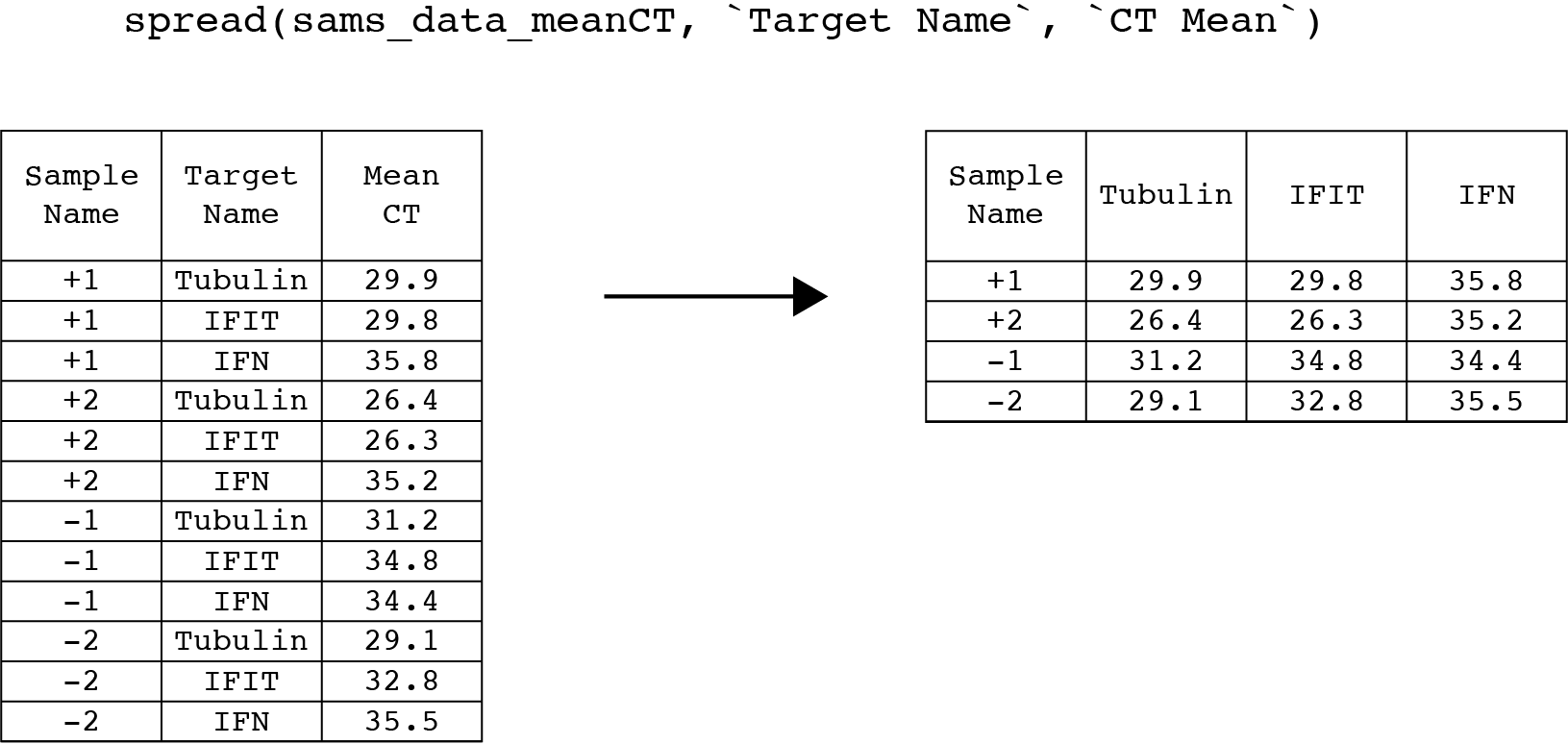
Make sure to view the new table using the viewer to ensure that spread() behaved correctly. It is often helpful to pick an observation, like Sample Name = +1, and follow the CT values as you manipulate the columns to convince yourself that the relationships in the data are maintained.

Now we can gather() the IFN and IFIT columns back into Target and CT columns. The first argument is the table that gets piped in from spread(). The next two arguments are new names for the key and value columns. We can take this opportunity to simplify our column names to Target and CT from Target Name and CT Mean. The remaining arguments are columns in the table that gather() should ignore (see the minus sign).

sams_data_meanCT <- sams_data %>% 
  #sams_data is piped to the first argument of select
  select("Sample Name", "Target Name", "CT Mean" = "Cт Mean") %>%
  #the output of select is piped to the first argument of filter
  filter(`Sample Name` != "007" & !is.na(`Sample Name`)) %>%
  #the output of filter is spiped to the first argument of mutate
  #To update instead of making a new column, we set the "new" column name to the same as the old column name
  mutate(`CT Mean` = as.numeric(`CT Mean`)) %>%
  #the output of mutate is the first (and only) argument to unique()
  unique() %>%
  #the output of unique is piped to the first argument of spread()
  spread(`Target Name`, `CT Mean`) %>%
  #the output of spread is piped to the first argument of gather()
  gather(Target, CT, -`Sample Name`, -Tubulin)
  #the output of gather is saved to sams_data_meanCT

Here is what gather() should look like with our data.

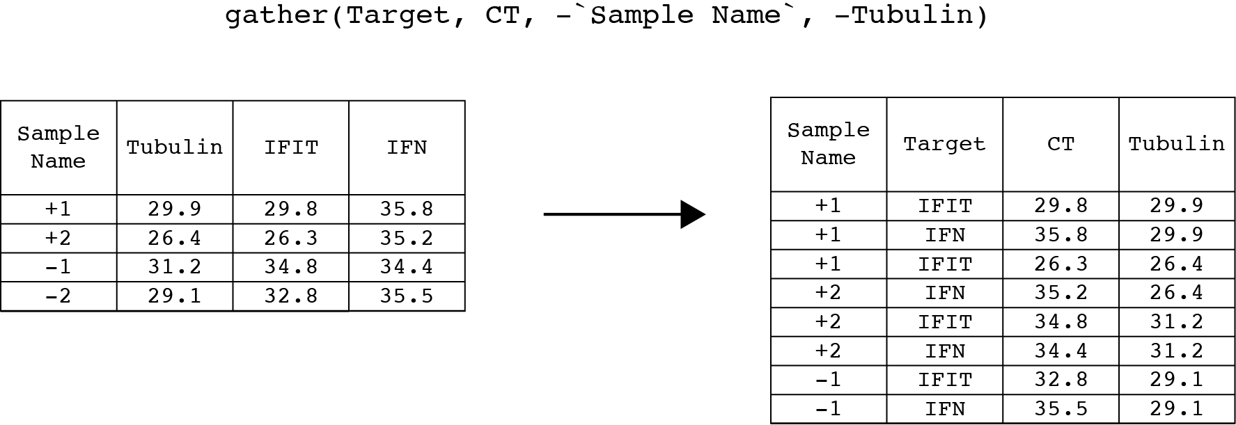
Once again, check the table in the viewer to make sure that gather() behaved as you expect.

Great! Now we can calculate the \(\Delta\)Ct. To calucate \(\Delta\)Ct, we can use the mutate() verb to subtract the values in the Tubulin column from the values in the CT column. As before, the first argument is the table (which we can pipe in). The second argument is new_column_name = function(old_column_name(s)). Since we are subtracting one column from another, our second argument will be deltaCt = CT - Tubulin.

sams_data_deltaCT <- sams_data_meanCT %>%
  mutate(deltaCT = CT - Tubulin)