R fridays #7: Fluorescence Anisotropy
Examining enzyme binding kinetics with fluorescence anisotropy
Today’s data and code were generously provided by Andrew Morris of the Ren lab. Fluorescence anisotropy is a technique to measure the binding of a fluorescent molecule to a protein of interest. If the fluorescent molecule is bound to the protein, it should have less freedom of movement in solution, resulting in the emitted light being more polarized. This allows for estimation of binding kinetics.
The data
Andrew used fluorescence anisotropy to measure binding of a mutant protein in different buffer conditions. He compared binding of the wild-type protein in 150mM NaCl in tris buffer to binding of the mutant protein in 50mM NaCl in tris buffer, 150mM NaCl in tris buffer, and 150mM NaCl in HEPES buffer. Today we will be working with data simulated from his experiment.
Loading in the data
Andrew read in his data using read_tsv() from the tidyverse package:
library(tidyverse)## ── Attaching packages ───────────────────────────────────────────────────────────────────────────────────────────────────────────────────────────────────────────────────────────── tidyverse 1.3.0 ──## ✓ ggplot2 3.2.1 ✓ purrr 0.3.3
## ✓ tibble 2.1.3 ✓ dplyr 0.8.3
## ✓ tidyr 1.0.0 ✓ stringr 1.4.0
## ✓ readr 1.3.1 ✓ forcats 0.4.0## ── Conflicts ──────────────────────────────────────────────────────────────────────────────────────────────────────────────────────────────────────────────────────────────── tidyverse_conflicts() ──
## x dplyr::filter() masks stats::filter()
## x dplyr::lag() masks stats::lag()nacl50_tris <- read_tsv("../../data/andrew_081619_50NaCl_Tris_noise.tsv")## Parsed with column specification:
## cols(
## NP = col_double(),
## ani = col_double()
## )nacl150_tris <- read_tsv("../../data/andrew_081619_150NaCl_Tris_noise.tsv")## Parsed with column specification:
## cols(
## NP = col_double(),
## ani = col_double()
## )nacl150_hepes <- read_tsv("../../data/andrew_081619_150NaCl_HEPES_noise.tsv")## Parsed with column specification:
## cols(
## NP = col_double(),
## ani = col_double()
## )wt <- read_tsv("../../data/andrew_081619_WT_noise.tsv")## Parsed with column specification:
## cols(
## NP = col_double(),
## ani = col_double()
## )There are two variables in the data. “ani” refers to the anisotropy value, which has already been baseline-corrected. “NP” refers to the concentration of the titrant in nanomolar.
Modeling independent binding
Andrew first tried modeling a 1 to 1 independent binding interaction between his ligand and protein by providing his data and the Michaelis-Menten equation to the nls() function in R. The nls() function will estimate parameters for a model given starting values and an equation for the model. There is also a specific function for estimating Michaelis-Menten parameters called SSmicmen(), but the equation is easy enough to write out.
The nls() function uses non-linear least squares regression to approximate a non-linear model by using linear models, and by iterating to successively improve estimation of the model parameters (see the wikipedia page here for a more detailed explanation).
Let’s check out the arguments needed for nls() by looking at the help page.
?nlsThe first argument is the equation for the model, in our case the Michaelis-Menten equation: \[V_0 = V_{max}\dfrac{[Substrate]}{[Substrate] + K_M}\] where \(V_0\) is the initial velocity of the reaction, \(V_{max}\) is the maximum velocity of the reaction, and \(K_M\) is the Michaelis-Menten constant.
The second argument is the data. The “ani” column in the data provides the \(V_0\) values for the equation, and the “NP” column is the Substrate concentration (\([Substrate]\)).
The third argument is the initial values that the nls() function will use to estimate the remaining variables in the equation (\(K_{M}\) and \(V_{max}\)). Our initial value for \(K_M\) will be half of the maximum \([Substrate]\), and the initial value for \(V_{max}\) (the anisotropy saturation value) will be the maximum of \(V_0\).
If the model has trouble converging, this indicates that our estimation of the apparent \(K_M\) may have been really off. In that case, we could plot the data to make a better guess about the true \(K_M\) to use as the initial value for nls().
model.nls <- nls(ani ~ Vm * NP/(K+NP),
                 data = wt,
                 start = list(K = max(wt$NP)/2, Vm = max(wt$ani)))

summary(model.nls)
##
## Formula: ani ~ Vm * NP/(K + NP)
##
## Parameters:
## Estimate Std. Error t value Pr(>|t|)
## K 368.07 54.09 6.805 1.29e-06 ***
## Vm 302.04 13.91 21.716 2.23e-15 ***
## ---
## Signif. codes: 0 '***' 0.001 '**' 0.01 '*' 0.05 '.' 0.1 ' ' 1
##
## Residual standard error: 19.39 on 20 degrees of freedom
##
## Number of iterations to convergence: 8
## Achieved convergence tolerance: 6.868e-06Andrew then used base R to plot his data and model
plot(wt)
lines(wt$NP, predict(model.nls), col = "red")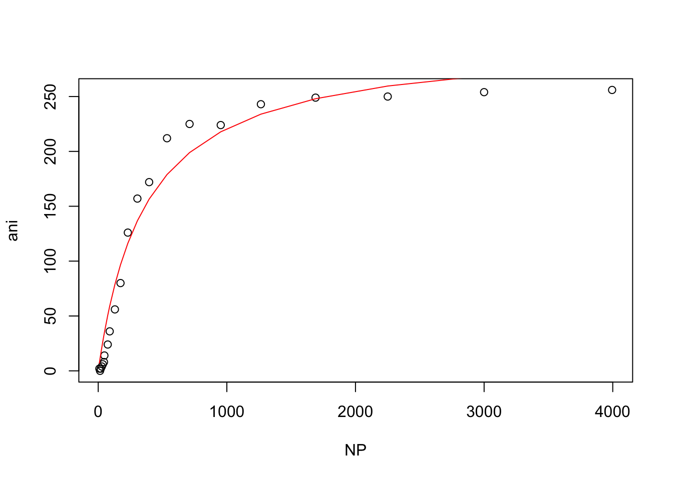
Andrew noticed that when his data is plotted on a log-scale there is a very sharp inflexion, which indicates that it likely does not fit a 1 to 1 independent binding model:
plot(log10(wt$NP), wt$ani)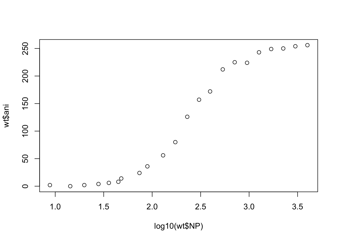
So his next step was to try to fit the Hill equation, which assumes cooperative binding.
Modeling cooperative binding
The Hill equation is given by: \[\theta = \dfrac{1}{(\dfrac{K_a}{[Substrate]})^n +1}\] where \(\theta\) is the fraction of the protein that is bound by the ligand, \(n\) is the hill coefficient, and \(K_a\) is the association constant.
To model his data using the Hill equation, Andrew first needed to normalize his data to maximum anisotropy (max(ani)) to treat anisotropy as the fractional occupancy of binding sites.
wt$ani <- wt$ani/max(wt$ani)Next Andrew fit the model assuming that \([Substrate]\) is approximately the same as \([unbound Substrate]\), and using initial values for \(K_a\) and \(n\) that he guessed from looking at his data.
hill_model.nls <- nls(ani ~ 1/(((Ka/NP)^n)+1),
                      data = wt,
                      start = list(Ka = 300, n=2))

summary(hill_model.nls)
##
## Formula: ani ~ 1/(((Ka/NP)^n) + 1)
##
## Parameters:
## Estimate Std. Error t value Pr(>|t|)
## Ka 249.15889 4.27001 58.35 <2e-16 ***
## n 1.83856 0.05118 35.92 <2e-16 ***
## ---
## Signif. codes: 0 '***' 0.001 '**' 0.01 '*' 0.05 '.' 0.1 ' ' 1
##
## Residual standard error: 0.01775 on 20 degrees of freedom
##
## Number of iterations to convergence: 5
## Achieved convergence tolerance: 5.86e-07Then he plotted the data as before.
plot(wt)
lines(wt$NP, predict(hill_model.nls), col = "red")
The plot and the Hill coefficient indicate that Andrew’s wild-type protein and ligand undergo cooperative binding.
Comparing wild-type and mutant protein binding
To compare the binding of the wild-type and mutant protein we could either copy and paste the code above for each buffer condition, or we could write a function to save time and decrease the possibility of copy-paste errors.
Here is a basic function called hello_world. Once hello_world is defined, it can be called by typing hello_world().
hello_world <- function(){
  print("This is a function")
}

hello_world()
## [1] "This is a function"Functions can also take arguments (think of functions you have already used, like read_tsv() and print()).
hello_world <- function(text){
  print(text)
}

hello_world("Biochemistry is cool")
## [1] "Biochemistry is cool"To learn more about functions and how they are useful in organizing and simplifying code, see the Functions chapter in R for Data Science by Hadley Wickham.
Here is a function to model the Hill equation and plot the result. Notice that the code is very similar to what we did in the previous section, except that the name of the dataset has been replaced with the argument name, conveniently called “dataset”.
hill <- function(dataset){
  #normalize the data to maximum anisotropy
  dataset$ani <- dataset$ani/max(dataset$ani)

  #fit the model using nls
  hill_model.nls <- nls(ani ~ 1/(((Ka/NP)^n)+1),
                      data = dataset,
                      start = list(Ka = 300, n=2))

  #print out a summary of the model
  summary(hill_model.nls)

  #plot the data and fit
  plot(dataset)
  lines(dataset$NP, predict(hill_model.nls), col = "red")
}
Now it is easy to call hill() on each dataset for the wt and mutant protein
hill(wt)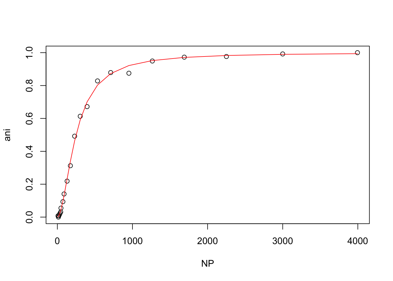
hill(nacl50_tris)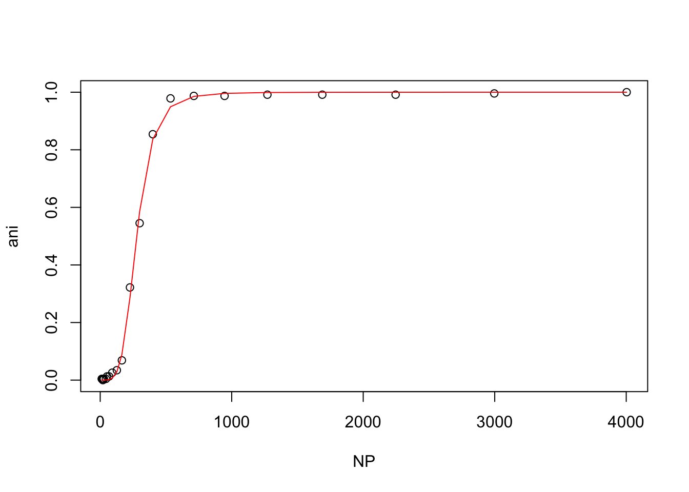
hill(nacl150_tris)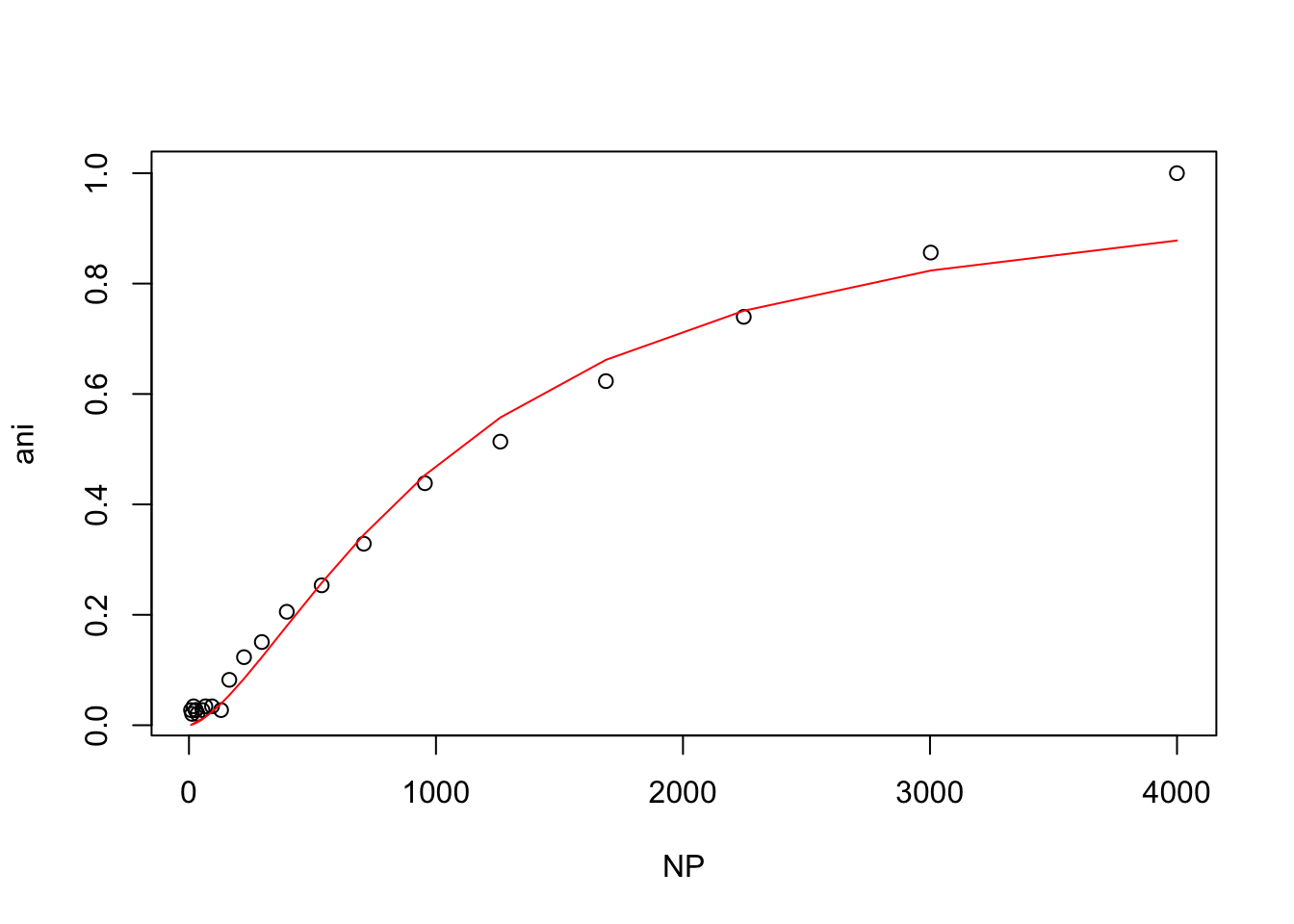
hill(nacl150_hepes)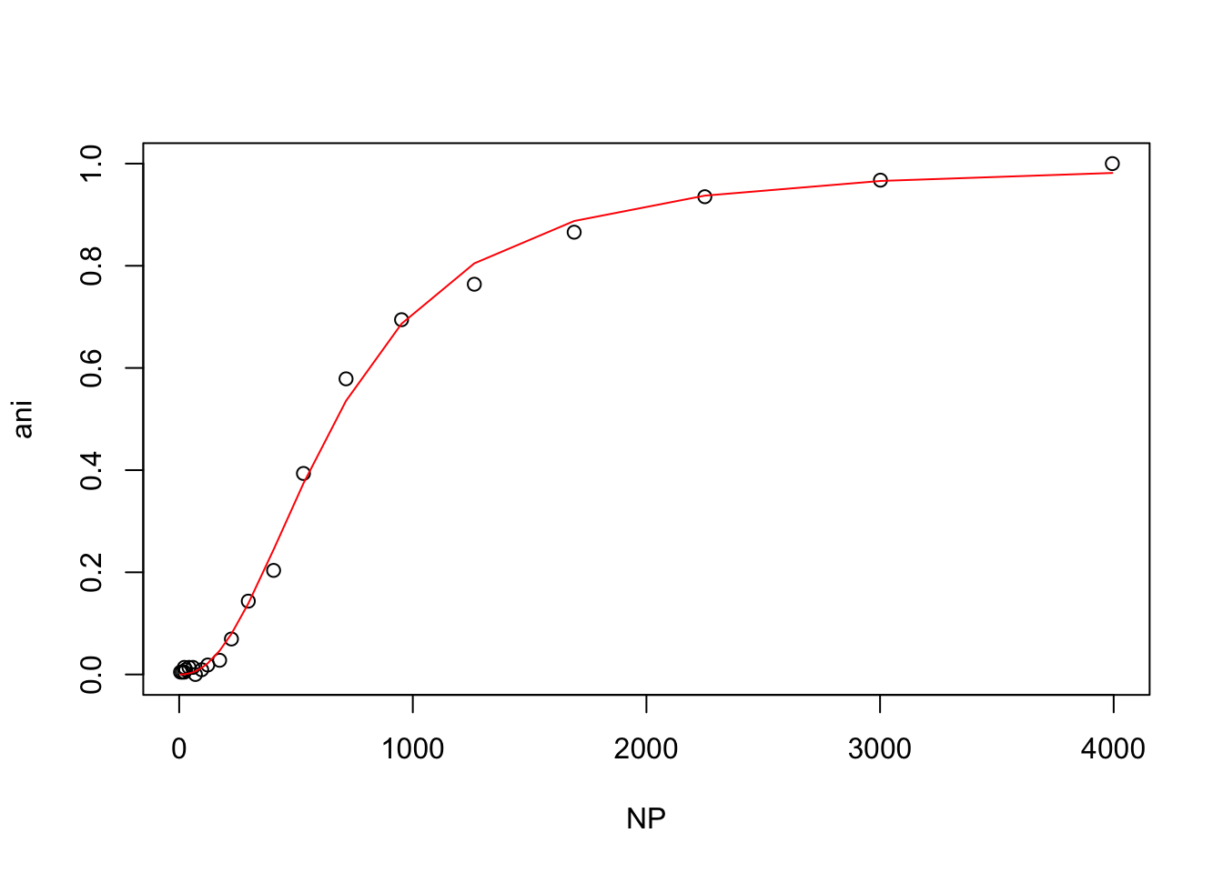
From these plots, t looks like the mutant protein binds the ligand more strongly than the wild-type at 50mM NaCl, but that higher NaCl concentrations inhibit binding.
Replicating this analysis using ggplot
ggplot2 has a layer called geom_smooth() that allows you to fit a model within your ggplot function. Here is an example using geom_smooth() to replicate the wt binding plot from above.
ggplot(wt, aes(NP, ani)) +
  geom_point() +
  geom_smooth(method = "nls",
               method.args=list(formula = y ~ 1/(((Ka/x)^n)+1),
                                start = list(Ka = 300, n = 2)),
               data = wt,
               color = "steelblue",
               se = FALSE)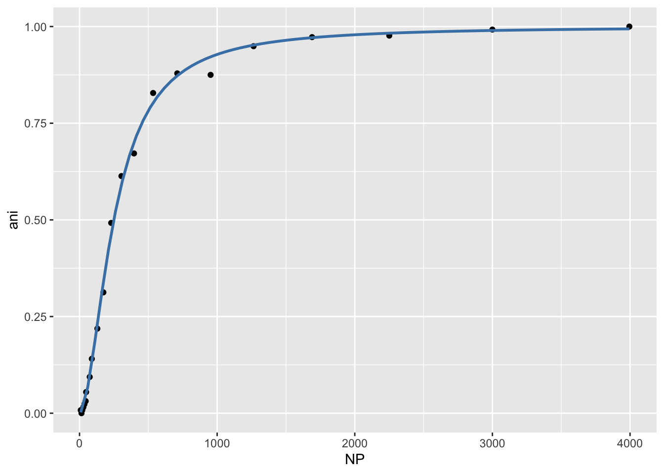
Wrap-up
Today we discovered that Andrew’s protein binds cooperatively to his ligand by modeling fluorescence anisotropy data using the Michaelis-Menten equation and the Hill equation. We also saw that the binding is inhibited at higher NaCl concentrations (150mM). We learned how to construct a function to simplify code, and we learned how to fit a model within a ggplot function.
As always, if you have any questions don’t hesitate to email me.