The experiment

The example dataset was simulated from an experiment comparing RNA expression levels from two conditions (treated and untreated) in a human monocyte cell line (THP1). The cells were treated with cGAMP, an agonist of the STING signaling pathway, to stimulate an innate immune response. The treatment was also performed in a timecourse, with 0 hours representing the untreated condition, and timepoints at 0.5, 4, and 16 hours post-treatment with cGAMP. Each condition has three biological replicates.

The data

RNA-seq data undergoes a series of processing steps before it can be visualized in R:

1. Quality control of reads (sequence length, GC content, adapter content, etc.)
2. Trimming adapters
3. Removal of PCR duplicates
4. Alignment to a reference genome/transcriptome
5. Quantification and normalization

The input data for this analysis is quantified and normalized RNA-seq expression data. The unit for the data is FPKM (fragments per kilobase per million), you can learn more about how this value was calculated from this helpful post. Specifically, Katie used Cuffdiff from the Cufflinks software to quantify and normalize her data, and the input file for this analysis is the “cds.fpkm_tracking” file from Cuffdiff.

Loading the data into R

Katie used the tidyverse packages to load and manipulate her data in R.

library(tidyverse)

## ── Attaching packages ───────────────────────────────────────────────────────────────────────────────────────────────────────────────────────────────────────────────────────────── tidyverse 1.3.0 ──

## ✓ ggplot2 3.2.1     ✓ purrr   0.3.3
## ✓ tibble  2.1.3     ✓ dplyr   0.8.3
## ✓ tidyr   1.0.0     ✓ stringr 1.4.0
## ✓ readr   1.3.1     ✓ forcats 0.4.0

## ── Conflicts ──────────────────────────────────────────────────────────────────────────────────────────────────────────────────────────────────────────────────────────────── tidyverse_conflicts() ──
## x dplyr::filter() masks stats::filter()
## x dplyr::lag()    masks stats::lag()

Specifically, she used the read_csv() function to read in her data and the select() function to select columns that she was interested in. She connected these two commands with a pipe (%>%) to send the output of read_tsv() to the first argument of select().

rna_seq <- read_csv("../../data/katie_080919_noise.csv") %>%
  select(gene_short_name, THP1_0H_1_1_FPKM, THP1_0H_2_1_FPKM, THP1_0H_3_1_FPKM,
         THP1_0_5H_1_1_FPKM, THP1_0_5H_2_1_FPKM, THP1_0_5H_3_1_FPKM,
         THP1_4H_1_1_FPKM, THP1_4H_2_1_FPKM, THP1_4H_3_1_FPKM, 
         THP1_16H_1_1_FPKM, THP1_16H_2_1_FPKM, THP1_16H_3_1_FPKM)

## Parsed with column specification:
## cols(
##   .default = col_double(),
##   class_code = col_character(),
##   nearest_ref_id = col_character(),
##   length = col_character(),
##   coverage = col_character(),
##   THP1_0H_1_1_status = col_character(),
##   THP1_0H_3_1_status = col_character(),
##   THP1_0_5H_2_1_status = col_character(),
##   THP1_16H_1_1_status = col_character(),
##   THP1_16H_3_1_status = col_character(),
##   THP1_4H_2_1_status = col_character(),
##   THP1_0H_1_2_status = col_character(),
##   THP1_0H_3_2_status = col_character(),
##   THP1_0_5H_2_2_status = col_character(),
##   THP1_16H_1_2_status = col_character(),
##   THP1_16H_3_2_status = col_character(),
##   THP1_4H_2_2_status = col_character(),
##   THP1_0H_2_1_status = col_character(),
##   THP1_0_5H_1_1_status = col_character(),
##   THP1_0_5H_3_1_status = col_character(),
##   THP1_16H_2_1_status = col_character()
##   # ... with 8 more columns
## )

## See spec(...) for full column specifications.

The columns she selected are the gene name (gene_short_name) and the FPKM values for all of her timepoints and conditions. THP1_0H_1_1_FPKM refers to biological replicate 1 of the unstimulated condition, THP1_0H_2_1_FPKM referse to replicate 2, and so on.

Cleaning the data

After loading in the data, Katie noticed that some genes had multiple FPKM values for the same experiment. This is due to different transcript isoforms. She chose to handle this situation by choosing the maximum FPKM value for a given gene. Another solution would have been to use the sum of all isoform FPKMs for a given gene. Either way, decisions like this are important to note in a methods section when the data is published.

Katie used summarize_all() which is a version of the summarize() dplyr function that we’ve covered in previous R fridays. summarize_all() applies a summarizing function (like max or mean) to every variable (column). Check out the commented code below to see how summarize_all() simplified the code compared to using just summarize().

expressiondata_max <- rna_seq %>%
  group_by(gene_short_name) %>%
  summarize_all(max)


# expressiondata_max <- rna_seq %>%
#   group_by(gene_short_name) %>%
#   summarize(THP1_0H_1_1_FPKM = max(THP1_0H_1_1_FPKM), 
#             THP1_0H_2_1_FPKM = max(THP1_0H_2_1_FPKM), 
#             THP1_0H_3_1_FPKM = max(THP1_0H_3_1_FPKM),
#             THP1_0_5H_1_1_FPKM = max(THP1_0_5H_1_1_FPKM),
#             THP1_0_5H_2_1_FPKM = max(THP1_0_5H_2_1_FPKM),
#             THP1_0_5H_3_1_FPKM = max(THP1_0_5H_3_1_FPKM),
#             THP1_4H_1_1_FPKM = max(THP1_4H_1_1_FPKM),
#             THP1_4H_2_1_FPKM = max(THP1_4H_2_1_FPKM),
#             THP1_4H_3_1_FPKM = max(THP1_4H_3_1_FPKM),
#             THP1_16H_1_1_FPKM = max(THP1_16H_1_1_FPKM),
#             THP1_16H_2_1_FPKM = max(THP1_16H_2_1_FPKM),
#             THP1_16H_3_1_FPKM = max(THP1_16H_3_1_FPKM))

Then Katie wanted to remove lowly-expressed genes. Removal of lowly-expressed genes can increase statistical power when looking for differential expression by decreasing the number of tests performed, and thus decreasing the multiple testing correction. Multiple R packages implement methods of removing lowly expressed genes, such as DEseq and edgeR. For this initial exploratory analysis though, Katie decided to simply threshold the genes by FPKM. She calculated the total FPKM value for each gene among all conditions, and kept genes with a total FPKM > 12.

expressiondata <- expressiondata_max %>%
  mutate(rowsum_uniq = rowSums(.[2:13])) %>%
  filter(rowsum_uniq > 12)

Lastly, Katie log2-transformed the FPKM values to bring them closer to a normal distribution. She used mutate_at() which is similar to summarize_all(), except that you can specify which variables to you want to apply the function to.

expressiondata_log <- expressiondata %>%
  mutate_at(2:13, log2)

Exploring the data

Katie next compared the FPKM values in the different conditions to see whether the treatment had any effect on gene expression.

To do this she transformed the data into a “narrow” format using gather(), and then added a grouping variable for each timepoint (see this post for a more detailed explanation). Then she calculated the mean expression for each gene among the biological replicates, and then spread() the data back into a wide format.

average_expression <- expressiondata_log %>%
  #removing an unnecessary variable
  select(-rowsum_uniq) %>%
  gather(key = sample, value = expression, -gene_short_name) %>%
  mutate(timepoint = str_extract(string = sample, pattern = "THP1_[^H]*H")) %>%
  group_by(gene_short_name, timepoint) %>%
  summarize(meanexpression = mean(expression)) %>%
  #putting the data back into a wide format
  spread(key = timepoint, value = meanexpression)

From this data format, it is easy to compare different conditions using ggplot:

ggplot(average_expression, aes(THP1_0H, THP1_16H)) +
  geom_point()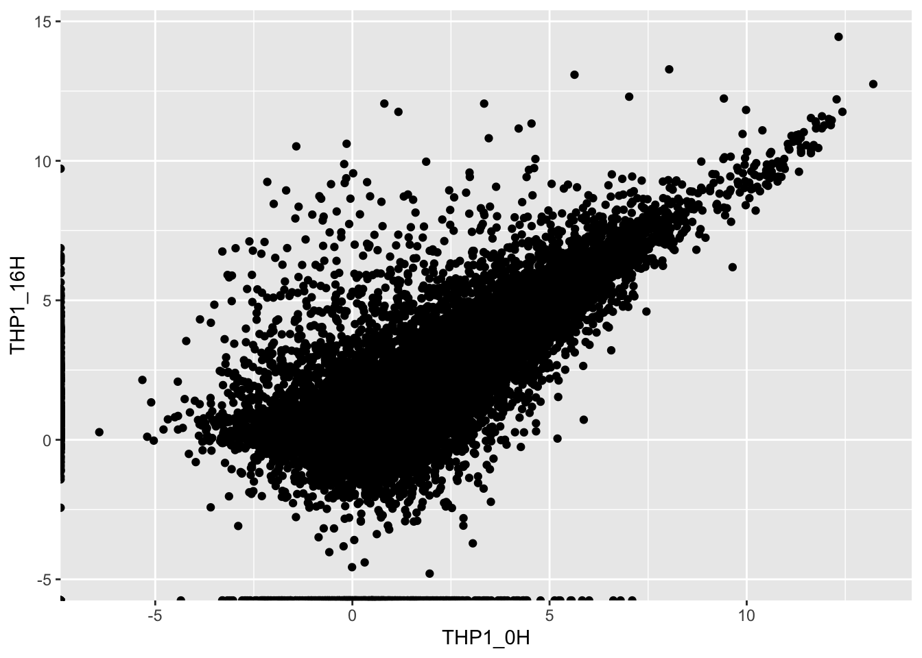

Great! There are multiple genes with higher or lower expression after 16 hours of treatment with cGAMP. We can construct plots comparing each timepoint to the untreated condition, and then stitch them together using the ggarrange() function from a package called ggpubr. I also added the setting alpha = 0.5 to the geom_point() layer to address the over-plotting.

library(ggpubr)

## Loading required package: magrittr

## 
## Attaching package: 'magrittr'

## The following object is masked from 'package:purrr':
## 
##     set_names

## The following object is masked from 'package:tidyr':
## 
##     extract

hour0.5 <- ggplot(average_expression, aes(THP1_0H, THP1_0_5H)) +
  geom_point(alpha = 0.5)

hour4 <- ggplot(average_expression, aes(THP1_0H, THP1_4H)) +
  geom_point(alpha = 0.5)

hour16 <- ggplot(average_expression, aes(THP1_0H, THP1_16H)) +
  geom_point(alpha = 0.5)

timepoints <- ggarrange(hour0.5, hour4, hour16,
                    labels = c("A", "B", "C"),
                    ncol = 3)
timepoints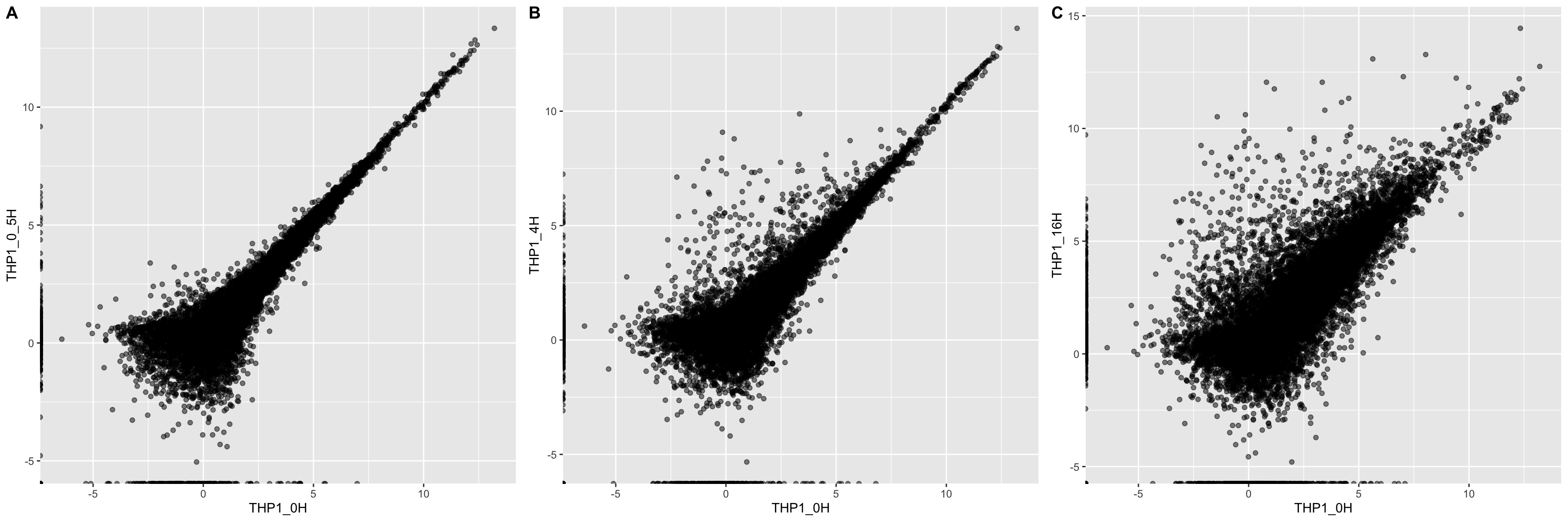

From this brief data cleaning and visualization, we can see that many different genes are differentially expressed upon treatment with cGAMP over time.

Some future steps might be to perform hypothesis testing to determine which genes are actually differentially expressed, and whether there are any patterns in gene expression across the timecourse.